Why do we need to explain our models?
Today, Machine Learning models are present in almost every industry, from drug discovery and medical diagnosis to stock market investment, fraud detection, and self-driving cars. At RTB House, we employ Machine Learning to optimize advertising campaigns for our clients.
However, most Machine Learning systems have a significant flaw: their decision-making processes are opaque. They are usually used like a black box: some data goes in, and predictions come out. While not all ML models have such a problem—some of them are relatively transparent—the more complex and deep the model is, the less we usually understand about how exactly it makes its predictions.
For some sectors, this can be a dealbreaker. E.g., models used by banks to calculate credit scores are legally required to be explainable. Explainability is also critical in the medical, legal, and automotive industries.
Understanding how our models ‘think’ can also help us improve them. If we could know how our features are influencing the model’s output, we could select those features better, transform them to give our model more significant information or find out that our model overfits some specific signal and debug it.
Fortunately, there is an entire domain dedicated to explaining Machine Learning models. Explainable AI (or XAI) methods enable us to look into any model we want, regardless of their architecture, and see where they get their outputs from.
What exactly can we explain?
There are many different model explanation methods, but they are mainly divided into two categories: local and global level explanations.
Local methods explain the output of our models for a specific instance. For example, consider a bank customer who wants to know why they’ve got a low credit score. Using local explanation methods like SHAP or LIME, we can check how factors such as age, earnings, or gender influenced the score calculated by the model. Other local-level methods, like Ceteris Paribus, allow us to explore hypothetical scenarios, such as how the score would change if the customer had a different gender or higher disposable income.
Global methods, on the other hand focus on the entire dataset and on how the features affect the model’s predictions in general. Feature importance scores can tell us which features most significantly impact the model’s predictions, while techniques like Partial Dependence Plots or Accumulated Local Effects can show how exactly those features contribute to those predictions. We can use them, for example, to see how age affects credit scores predicted by the model across all customers, highlighting trends that apply universally rather than to individual cases.
Explanation methods we use
Our main motivation for implementing Explainable AI methods in our system was to assist our researchers with feature engineering and model improvement. Since analyzing outputs for individual data instances is not necessary for us, we opted not to incorporate local explanation methods. Instead, our Model Explainer offers several global explanation methods:
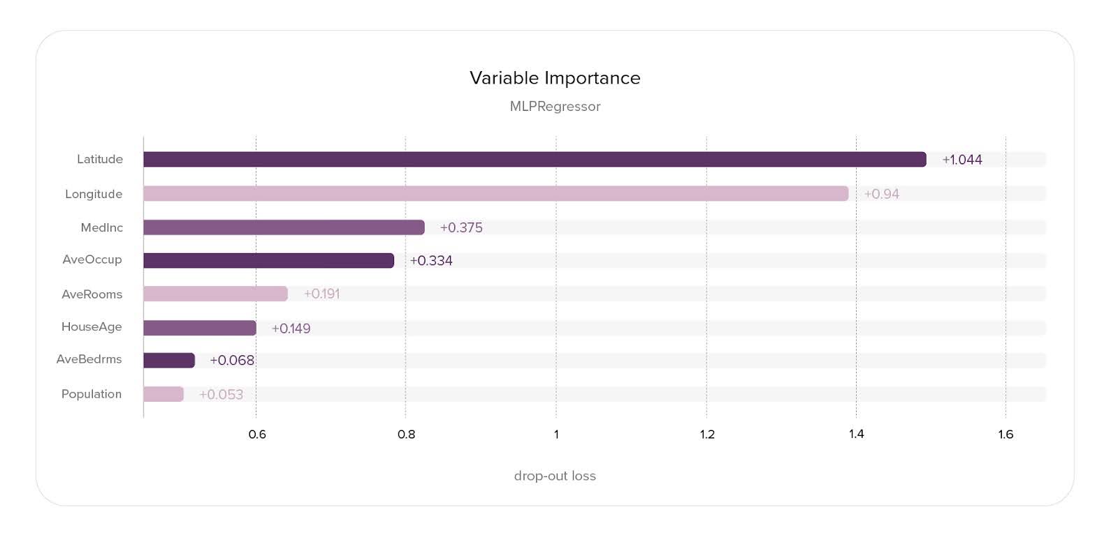
Feature Importance—These methods assign a value to each feature based on its importance to the model’s final output. There are various ways to calculate it. One of the simplest methods: Permutation Feature Importance is calculated by measuring model performance degradation when a feature’s values are shuffled within the dataset. Other popular methods use SHAP Values (which are used both at the local and global level explanation methods). In our Model Explainer, we implemented Expected Gradients Feature Importance, which is a method that approximates SHAP Values-based Feature Importance, but is much faster to calculate.
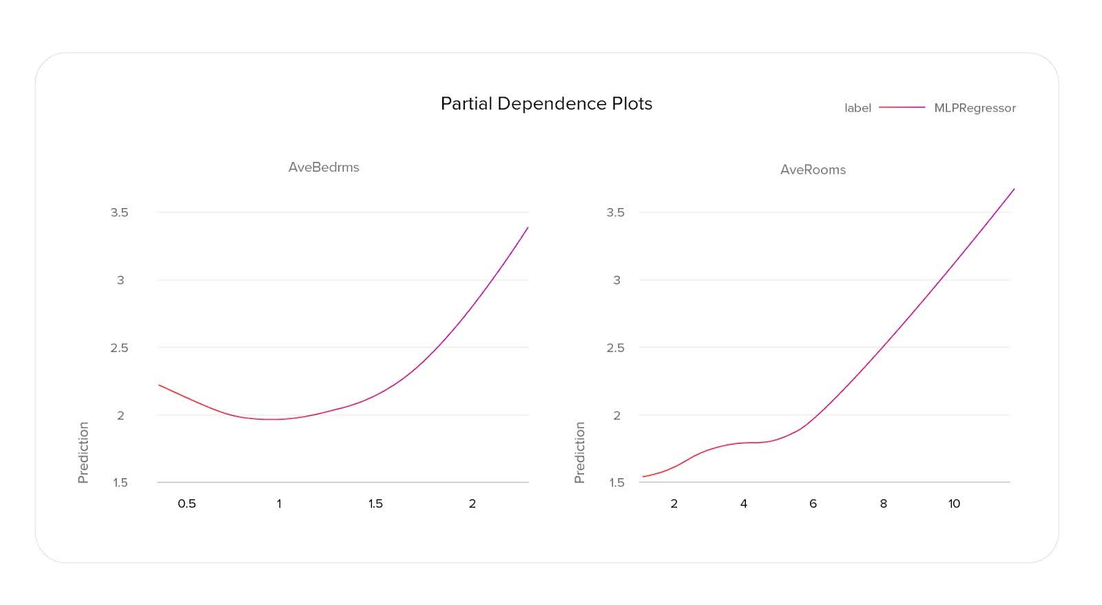
Partial Dependence Plots show us how the values of that feature correlate with the model’s output. To generate a PDP, we select a range of feature values, create modified datasets by substituting the original feature values with these selected values, and then calculate the average model prediction for each dataset. With such plots, we can see how an output is correlated with features. PDP can tell us if that correlation is more linear, logarithmic, or maybe more complex.
Accumulated Local Effects—One of the major disadvantages of PDP is that it doesn’t work well when features are correlated. ALE eliminates that problem. Instead of substituting feature values in the entire dataset with each of the selected values, to calculate ALE, we first divide the dataset into buckets based on the values of that feature. Then, for each datapoint, we substitute the feature value first with the left bucket boundary and then with the right, subtracting the former predictions from the latter to calculate local effects. The cumulative sum of these local effects provides the accumulated local effects.
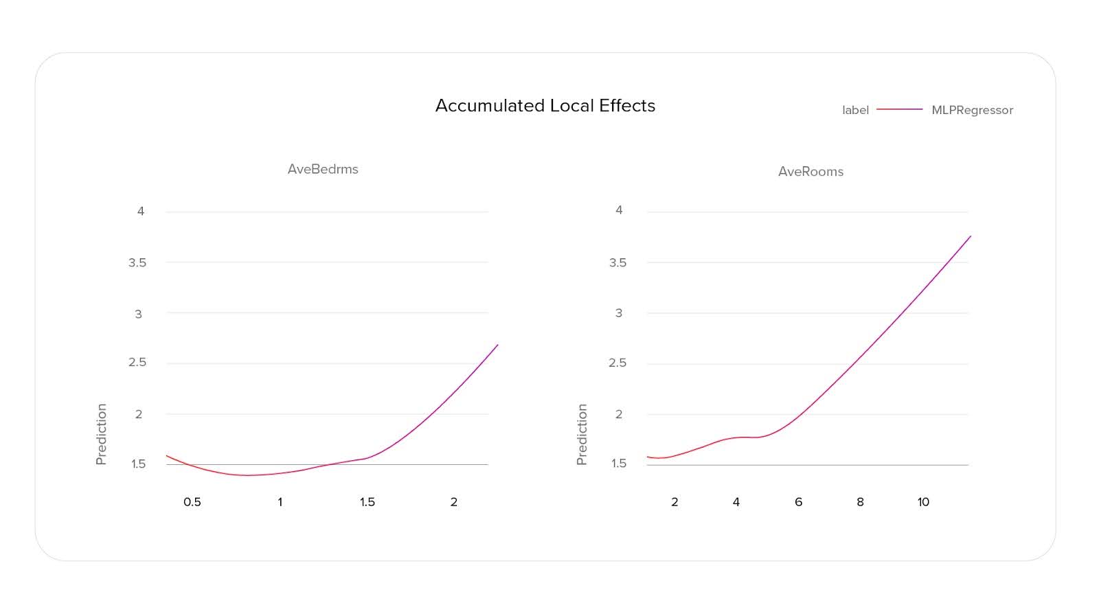
Since we make only small changes to our data points, we are not generating out-of-distribution samples in our modified datasets by doing this. That means the method works well even when features are correlated (unlike PDP). But there is also a downside: this method requires our feature values to have an order. It’s more complicated to calculate ALE for categorical features. That’s why, in our Model Explainer, we also left Partial Dependence Plots.
Some other interesting methods
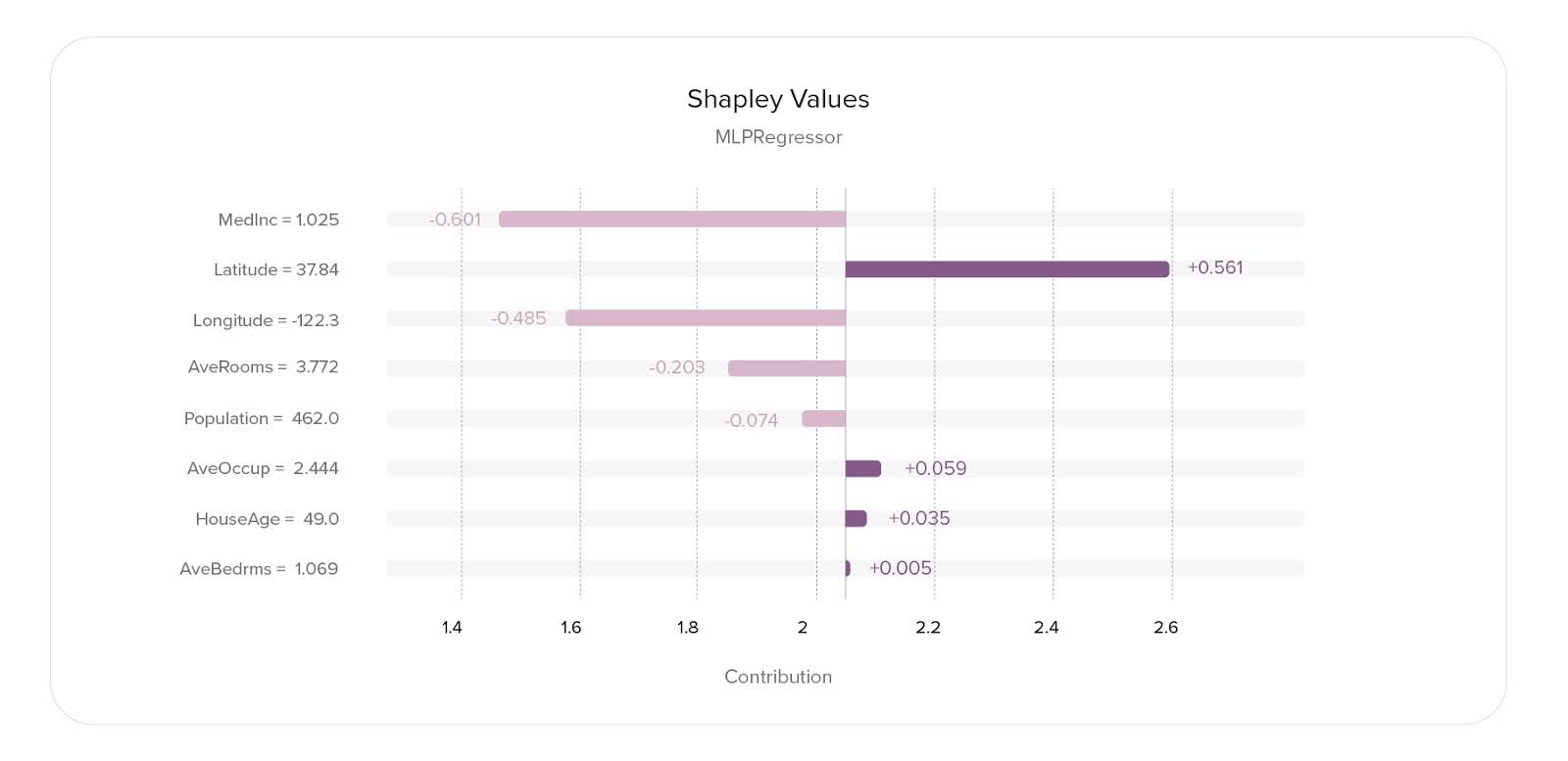
SHAP (SHapley Additive exPlanations)—This is a local explanation method derived from Shapley values, which were introduced in 1951 by the Nobel laureate in economics, Lloyd Shapley. Originally used to determine fair reward distribution in coalitional games, where a group of players achieves a greater reward together than individually, Shapley values can analogously measure the contribution of each feature (treated as players) to a model’s prediction. This approach helps us understand how each feature value influences the model’s output. It can also be used to calculate the importance of global-level features. The easiest way to do it is to take an average modulus of a SHAP value of a feature over the entire dataset.
Feature Interactions—There is a popular saying about collaboration: “One plus one is more than two.” This can also be applied to the features of a Machine Learning model. When combining two (or more) features inside our model, its predictions are based not only on the values of individual features but also on their interactions. For instance, imagine a simple model used to predict a price of an apartment, with size and neighborhood as its features. When looking at those features individually, a model would probably guess that there is a positive correlation between the size of an apartment and its price. Similarly, the better the neighborhood an apartment is located in, the higher its value is. Models predictions would consist of some constant base factor, some term based on the size, plus a neighborhood “bonus.” But if our model could look at both features together, there would also be a term of interaction between those features. For instance, different neighborhoods can have different average prices per square meter. Moreover, in some neighborhoods, large apartments can be disproportionally more expensive. We can examine how the features interact inside our model with different methods of calculating Feature Interactions. This complex method can be particularly useful when we are working with models that have some specific architectures like FFMs or when we want to use a simpler model and we need to use feature engineering to manually create some new features.
How do we use Explainable AI in our system?
As we transition into a cookieless world, feature engineering becomes especially important to us. We are redesigning our models, training, and feature extraction pipelines to adapt to the new privacy-oriented environment. In order to help our Machine Learning researchers improve existing models and design new ones, we revisited our suite of explainable AI tools.
Previously, we used two separate tools—one for calculating feature importance and another for generating partial dependence plots. These tools required manual activation for each model, with calculations taking several hours to complete and interfaces that were not friendly for new users. To address those issues, we developed a new Model Explainer app that integrates Feature Importance, Partial Dependence Plots, and added Accumulated Local Effects, which are more suited to the nature of our data.
Now, all explanation methods are regularly and automatically calculated for every production and experimental model in our system. Our ML researchers can access model explanations at any time through an intuitive web app, eliminating the need to manually initiate calculations and wait for results.
Summary
Explainable AI provides us with many different tools to explain our models. With local methods, we can analyze our model’s behavior on a specific sample, while with global ones, we can better understand trends in our model’s predictions. By defining our goals, selecting proper XAI methods for our needs, and implementing them into our system, we can get an insight into our models, explore (and eliminate) potential biases, and improve our Machine Learning pipeline.
Further read
- Great book about XAI (by Przemyslaw Biecek and Tomasz Burzykowski): https://ema.drwhy.ai/
- Another great book about XAI (by Christoph Molnar): https://christophm.github.io/interpretable-ml-book/
- Python and R package for explaining ML models (by MI2.AI): https://dalex.drwhy.ai/
- Original paper about SHAP explanation (by Scott Lundberg and Su-In Lee): https://arxiv.org/abs/1705.07874
- Paper about Expected Gradients Feature Importance (by Gabriel Erion, Joseph D. Janizek, Pascal Sturmfels, et al.): https://arxiv.org/abs/1906.10670